线性回归
线性回归(Linear Regression)是利用线性回归方程的最小二乘函数对一个或多个自变量和因变量之间关系进行建模的一种回归分析方法。其中只有一个自变量的情况称为简单回归,大于一个自变量的情况叫做多元回归。
相关假设
- 自变量与因变量间满足线性关系
- 误差项($\varepsilon$)之间应相互独立
- 误差项($\varepsilon$)的方差应为常数
- 误差项($\varepsilon$)应呈正态分布
- 自变量之间应相互独立
说明:若待训练的数据不满足上述假设,则线性回归的效果会比较差。可通过相关指数$R^2$来量化回归效果,$R^2$越接近于1,表示回归的效果越好。[]
数学描述
- 数据$\left( y_i,x_{i1},\cdots ,x_{ip} \right) ,i=1,\cdots ,n$
表示共用$n$个样本,每个样本共用$p$个特征。
- 模型
其中,$x_i,y_i$分别为已知的自变量与因变量,$\varepsilon _i$表示第$i$个样本的预测误差,$\theta$为待学习的模型参数
损失函数
通过最小化损失函数(MSE-均方差)来学习线性回归模型的参数
(主要是基于误差项($\varepsilon$)呈正态分布的假设,利用极大似然估计求解正态分布相关参数,从而得到MSE)
上述损失函数为凸函数,具有全局最优解。
求解方法
-
正规方程法(normal equation)
不需要设定学习率,不需要迭代,当样本数/特征数很大时,计算会很慢。
$\frac{\partial J\left( \theta \right)}{\partial \theta}=0\Rightarrow \theta =\left( X^TX \right) ^{-1}X^Ty$
当$ X^TX $不可逆时
- 可能存在线性相关的特征,需删除冗余的特征
- 可能特征过多(样本数<=特征数)导致,需删除一些特征,或使用正则化的方法
- 使用伪逆代替其逆矩阵[numpy.linalg.pinv()]
-
梯度下降法
通过设定学习率,不断的迭代,最终确定待求参数。当样本数/特征数很大时,依然工作良好。
实战
预测A股上市公司5天后的收盘价
数据文件为000001.csv
!!线性模型不太合理,仅做参考说明!!
import numpy as np # 数学计算
import pandas as pd # 数据处理, 读取 CSV 文件 (e.g. pd.read_csv)
import matplotlib.pyplot as plt
from datetime import datetime as dt
# 你可以使用如下的方法下载某一个公司的股票交易历史
# 000001 为平安银行
# 如果你还没有安装, 可以使用 pip install tushare 安装tushare python包
#import tushare as ts
#df = ts.get_hist_data('000001')
#print(df)
#df.to_csv('000001.csv')
df = pd.read_csv('./000001.csv')
print(np.shape(df))
df.head()
(611, 14)
| date | open | high | close | low | volume | price_change | p_change | ma5 | ma10 | ma20 | v_ma5 | v_ma10 | v_ma20 | |
|---|---|---|---|---|---|---|---|---|---|---|---|---|---|---|
| 0 | 2019-05-30 | 12.32 | 12.38 | 12.22 | 12.11 | 646284.62 | -0.18 | -1.45 | 12.366 | 12.390 | 12.579 | 747470.29 | 739308.42 | 953969.39 |
| 1 | 2019-05-29 | 12.36 | 12.59 | 12.40 | 12.26 | 666411.50 | -0.09 | -0.72 | 12.380 | 12.453 | 12.673 | 751584.45 | 738170.10 | 973189.95 |
| 2 | 2019-05-28 | 12.31 | 12.55 | 12.49 | 12.26 | 880703.12 | 0.12 | 0.97 | 12.380 | 12.505 | 12.742 | 719548.29 | 781927.80 | 990340.43 |
| 3 | 2019-05-27 | 12.21 | 12.42 | 12.37 | 11.93 | 1048426.00 | 0.02 | 0.16 | 12.394 | 12.505 | 12.824 | 689649.77 | 812117.30 | 1001879.10 |
| 4 | 2019-05-24 | 12.35 | 12.45 | 12.35 | 12.31 | 495526.19 | 0.06 | 0.49 | 12.396 | 12.498 | 12.928 | 637251.61 | 781466.47 | 1046943.98 |
股票数据的特征
- date:日期
- open:开盘价
- high:最高价
- close:收盘价
- low:最低价
- volume:成交量
- price_change:价格变动
- p_change:涨跌幅
- ma5:5日均价
- ma10:10日均价
- ma20:20日均价
- v_ma5:5日均量
- v_ma10:10日均量
- v_ma20:20日均量
# 将每一个数据的键值的类型从字符串转为日期

df['date'] = pd.to_datetime(df['date'])
df = df.set_index('date')
# 按照时间升序排列
df.sort_values(by=['date'], inplace=True, ascending=True)
df.tail()
| open | high | close | low | volume | price_change | p_change | ma5 | ma10 | ma20 | v_ma5 | v_ma10 | v_ma20 | |
|---|---|---|---|---|---|---|---|---|---|---|---|---|---|
| date | |||||||||||||
| 2019-05-24 | 12.35 | 12.45 | 12.35 | 12.31 | 495526.19 | 0.06 | 0.49 | 12.396 | 12.498 | 12.928 | 637251.61 | 781466.47 | 1046943.98 |
| 2019-05-27 | 12.21 | 12.42 | 12.37 | 11.93 | 1048426.00 | 0.02 | 0.16 | 12.394 | 12.505 | 12.824 | 689649.77 | 812117.30 | 1001879.10 |
| 2019-05-28 | 12.31 | 12.55 | 12.49 | 12.26 | 880703.12 | 0.12 | 0.97 | 12.380 | 12.505 | 12.742 | 719548.29 | 781927.80 | 990340.43 |
| 2019-05-29 | 12.36 | 12.59 | 12.40 | 12.26 | 666411.50 | -0.09 | -0.72 | 12.380 | 12.453 | 12.673 | 751584.45 | 738170.10 | 973189.95 |
| 2019-05-30 | 12.32 | 12.38 | 12.22 | 12.11 | 646284.62 | -0.18 | -1.45 | 12.366 | 12.390 | 12.579 | 747470.29 | 739308.42 | 953969.39 |
# 检测是否有缺失数据 NaNs

df.dropna(axis=0 , inplace=True)
df.isna().sum()
open            0
high            0
close           0
low             0
volume          0
price_change    0
p_change        0
ma5             0
ma10            0
ma20            0
v_ma5           0
v_ma10          0
v_ma20          0
dtype: int64
# K线图
Min_date = df.index.min()
Max_date = df.index.max()
print ("First date is",Min_date)
print ("Last date is",Max_date)
print (Max_date - Min_date)
First date is 2016-11-29 00:00:00
Last date is 2019-05-30 00:00:00
912 days 00:00:00
from plotly import tools
from plotly.graph_objs import *
from plotly.offline import init_notebook_mode, iplot, iplot_mpl
init_notebook_mode()
import plotly.plotly as py
import plotly.graph_objs as go

trace = go.Ohlc(x=df.index, open=df['open'], high=df['high'], low=df['low'], close=df['close'])
data = [trace]
# iplot(data, filename='simple_ohlc') # K线图输出
# 线性回归
from sklearn.linear_model import LinearRegression
from sklearn import preprocessing
# 创建新的列, 包含预测值, 根据当前的数据预测5天以后的收盘价
num = 5 # 预测5天后的情况
df['label'] = df['close'].shift(-num) # 预测值

print(df.shape)
(611, 14)
# 丢弃 'label', 'price_change', 'p_change', 不需要它们做预测
Data = df.drop(['label', 'price_change', 'p_change'],axis=1)
Data.tail()
| open | high | close | low | volume | ma5 | ma10 | ma20 | v_ma5 | v_ma10 | v_ma20 | |
|---|---|---|---|---|---|---|---|---|---|---|---|
| date | |||||||||||
| 2019-05-24 | 12.35 | 12.45 | 12.35 | 12.31 | 495526.19 | 12.396 | 12.498 | 12.928 | 637251.61 | 781466.47 | 1046943.98 |
| 2019-05-27 | 12.21 | 12.42 | 12.37 | 11.93 | 1048426.00 | 12.394 | 12.505 | 12.824 | 689649.77 | 812117.30 | 1001879.10 |
| 2019-05-28 | 12.31 | 12.55 | 12.49 | 12.26 | 880703.12 | 12.380 | 12.505 | 12.742 | 719548.29 | 781927.80 | 990340.43 |
| 2019-05-29 | 12.36 | 12.59 | 12.40 | 12.26 | 666411.50 | 12.380 | 12.453 | 12.673 | 751584.45 | 738170.10 | 973189.95 |
| 2019-05-30 | 12.32 | 12.38 | 12.22 | 12.11 | 646284.62 | 12.366 | 12.390 | 12.579 | 747470.29 | 739308.42 | 953969.39 |
X = Data.values
X = preprocessing.scale(X)
X = X[:-num]

df.dropna(inplace=True)
Target = df.label
y = Target.values

print(np.shape(X), np.shape(y))
(606, 11) (606,)
# 将数据分为训练数据和测试数据
X_train, y_train = X[0:550, :], y[0:550]
X_test, y_test = X[550:, -51:], y[550:606]
print(X_train.shape)
print(y_train.shape)
print(X_test.shape)
print(y_test.shape)
(550, 11)
(550,)
(56, 11)
(56,)
lr = LinearRegression()
lr.fit(X_train, y_train)
lr.score(X_test, y_test) # 使用绝对系数 R^2 评估模型
0.049300406483855586
# 做预测

X_Predict = X[-num:]
Forecast = lr.predict(X_Predict)
print(Forecast)
print(y[-num:])
print(X_Predict)
[12.5019651  12.45069629 12.56248765 12.3172638  12.27070154]
[12.35 12.37 12.49 12.4  12.22]
[[ 1.33981111  1.19832101  1.02012019  1.10423258 -0.09374448  1.13748585
   1.1738002   1.73046344 -0.1920154   0.27170906  0.26317999]
 [ 0.97813252  0.96110571  0.98222502  1.03191402 -0.38046451  1.14768664
   1.14222724  1.66534722 -0.17460951 -0.00658067  0.23823498]
 [ 1.00985871  1.07667214  1.09591053  1.10423258 -0.46913789  1.15661234
   1.11709775  1.60680839 -0.35109762 -0.07844506  0.26392379]
 [ 1.11772776  0.97935304  0.99485674  1.07793492 -0.83038427  1.09030716
   1.10421083  1.5305106  -0.58481498 -0.17720161  0.17914381]
 [ 0.9083349   0.88811639  0.92538227  0.95959547 -0.57247177  1.01890159
   1.11258733  1.46934081 -0.57232128 -0.36458186  0.10403438]]
# 画预测结果
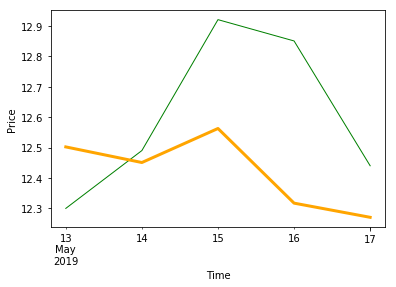
# 预测 2019-05-13 到 2019-05-17 , 一共 5 天的收盘价
trange = pd.date_range('2019-05-13', periods=num, freq='d')
trange
DatetimeIndex(['2019-05-13', '2019-05-14', '2019-05-15', '2019-05-16',
               '2019-05-17'],
              dtype='datetime64[ns]', freq='D')
# 产生预测值dataframe
Predict_df = pd.DataFrame(Forecast, index=trange)
Predict_df.columns = ['forecast']
Predict_df
| forecast | |
|---|---|
| 2019-05-13 | 12.501965 |
| 2019-05-14 | 12.450696 |
| 2019-05-15 | 12.562488 |
| 2019-05-16 | 12.317264 |
| 2019-05-17 | 12.270702 |
# 将预测值添加到原始dataframe
df = pd.read_csv('./000001.csv')
df['date'] = pd.to_datetime(df['date'])
df = df.set_index('date')
# 按照时间升序排列
df.sort_values(by=['date'], inplace=True, ascending=True)
df_concat = pd.concat([df, Predict_df], axis=1)

df_concat = df_concat[df_concat.index.isin(Predict_df.index)]
df_concat.tail(num)
| open | high | close | low | volume | price_change | p_change | ma5 | ma10 | ma20 | v_ma5 | v_ma10 | v_ma20 | forecast | |
|---|---|---|---|---|---|---|---|---|---|---|---|---|---|---|
| 2019-05-13 | 12.33 | 12.54 | 12.30 | 12.23 | 741917.75 | -0.38 | -3.00 | 12.538 | 13.143 | 13.637 | 1107915.51 | 1191640.89 | 1211461.61 | 12.501965 |
| 2019-05-14 | 12.20 | 12.75 | 12.49 | 12.16 | 1182598.12 | 0.19 | 1.54 | 12.446 | 12.979 | 13.585 | 1129903.46 | 1198753.07 | 1237823.69 | 12.450696 |
| 2019-05-15 | 12.58 | 13.11 | 12.92 | 12.57 | 1103988.50 | 0.43 | 3.44 | 12.510 | 12.892 | 13.560 | 1155611.00 | 1208209.79 | 1254306.88 | 12.562488 |
| 2019-05-16 | 12.93 | 12.99 | 12.85 | 12.78 | 634901.44 | -0.07 | -0.54 | 12.648 | 12.767 | 13.518 | 971160.96 | 1168630.36 | 1209357.42 | 12.317264 |
| 2019-05-17 | 12.92 | 12.93 | 12.44 | 12.36 | 965000.88 | -0.41 | -3.19 | 12.600 | 12.626 | 13.411 | 925681.34 | 1153473.43 | 1138638.70 | 12.270702 |
# 画预测值和实际值

df_concat['close'].plot(color='green', linewidth=1)
df_concat['forecast'].plot(color='orange', linewidth=3)
plt.xlabel('Time')
plt.ylabel('Price')
plt.show()
# 理解模型
for idx, col_name in enumerate(['open', 'high', 'close', 'low', 'volume', 'ma5', 'ma10', 'ma20', 'v_ma5', 'v_ma10', 'v_ma20']):
    print("The coefficient for {} is {}".format(col_name, lr.coef_[idx]))
The coefficient for open is -0.7620771175521583
The coefficient for high is 0.8316702513661574
The coefficient for close is 0.24459501282378332
The coefficient for low is 1.0913280171403381
The coefficient for volume is 0.004368110601913278
The coefficient for ma5 is -0.30718399033267807
The coefficient for ma10 is 0.19367301956267854
The coefficient for ma20 is 0.24974050920896698
The coefficient for v_ma5 is 0.17428438827048187
The coefficient for v_ma10 is 0.08848099154182543
The coefficient for v_ma20 is -0.2779741616955218
参考
逻辑回归(对数几率回归)
逻辑回归(logistic regression)是一种分类算法。它假设数据服从伯努利分布,通过极大似然函数的方法,运用梯度下降来求解模型参数,从而达到将数据二分类的目的。
相关假设
- 样本标签值服从伯努利分布(0-1分布)
- 模型输出值表示样本为正例(1)的概率
数学描述
逻辑回归是一种对数线性模型,利用逻辑函数[$\phi \left( z \right) =\frac{1}{1+e^{-z}}$],将线性回归模型[$z=\theta ^Tx$]的预测值转化为分类任务对应的概率。
且
其中
表示样本$x$为正样本的概率,
表示样本$x$为负样本的概率,两者的比值$\frac{\phi \left( z \right)}{1-\phi \left( z \right)}$称为几率,由以上分析可知线性回归模型的输出拟合对数几率,即对数线性回归。因此,逻辑回归也叫对数几率回归。
综上,(二项)逻辑回归的数学模型为:(样本$x$为正样本或负样本的概率)
损失函数
通过最小化损失函数可求得逻辑回归的模型参数$\theta$。
首先不能像线性回归那样通过均方误差(MSE)定义逻辑回归的损失函数,MSE对逻辑回归模型来说不是一个凸函数,不好求解全局最优解。而最大似然作为逻辑回归模型的损失函数,易于求得参数的最优解(凸函数)。
由上面的数学模型,指定训练集的似然函数为
为了简化运算,对上式两边取对数得
现在需要找出一组$\theta$,使得$l\left( \theta \right)$的值最大。加一个负号后,就变成最小化负对数似然函数,即最终的逻辑回归的损失函数为
接下来,以某一个样本为例,其损失函数为: $J\left( \theta \right) =-y\ln \left( h_{\theta}\left( x;\theta \right) \right) -\left( 1-y \right) \ln \left( 1-h_{\theta}\left( x;\theta \right) \right) $
等价于
可视化分析
import matplotlib.pyplot as plt
import numpy as np

x = np.arange(0, 1, 0.01)
y1 = -np.log(x)
y2 = -np.log(1-x)
y3 = y1 + y2

plt.xlabel(r"$h_{\theta}\left( x;\theta \right)$")# (预测(正样本)概率)
plt.ylabel(r"$J\left( \theta \right)$")# (损失函数)
plt.plot(x, y1)
plt.plot(x, y2,'--')
plt.plot(x, y3,':')
plt.legend(['y=1','y=0','y'])

plt.show()
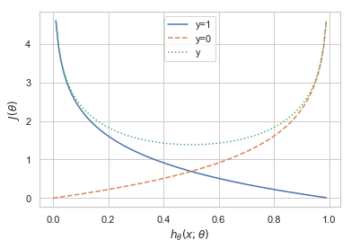
可以看出,如果样本的类别为1,估计值$h_{\theta}\left( x;\theta \right)$越接近1付出的损失越小,反之越大。
同理,如果样本的值为0的话,估计值$h_{\theta}\left( x;\theta \right)$越接近于0付出的损失越小,反之越大。
最后,利用梯度下降法最小化损失函数,从而求解逻辑回归的模型参数$\theta$
当样本量极大的时候,每次更新模型参数需要遍历整个数据集,会非常耗时,这时可以采用随机梯度下降法。即每次仅用一个样本点来更新模型参数。
三种梯度下降方法的比较
- 批量梯度下降BGD(Batch Gradient Descent):优点:会获得全局最优解,易于并行实现。缺点:更新每个参数时需要遍历所有的数据,计算量会很大并且有很多的冗余计算,导致当数据量大的时候每个参数的更新都会很慢。
- 随机梯度下降SGD:优点:训练速度快;缺点:准确率下降,并不是全局最优,不易于并行实现。它的具体思路是更新每一个参数时都是用一个样本来更新。(以高方差频繁更新,优点是使得sgd会跳到新的和潜在更好的局部最优解,缺点是使得收敛到局部最优解的过程更加的复杂。)
- small batch梯度下降:结合了上述两点的优点,每次更新参数时仅使用一部分样本,减少了参数更新的次数,可以达到更加稳定的结果,一般在深度学习中采用这种方法。
说明:上述三种梯度下降法的学习率都是固定的,可考虑Adam,动量法等优化方法动态改变学习率。
优缺点
优点:
- 形式简单,模型的可解释性非常好,特征的权重可以看到不同的特征对最后结果的影响
- 模型效果不错。在工程上是可以接受的(作为baseline),如果特征工程做的好,效果不会太差,并且特征工程可以大家并行开发,大大加快开发的速度
- 训练速度较快。分类的时候,计算量仅仅只和特征的数目相关。并且逻辑回归的分布式优化sgd发展比较成熟,训练的速度可以通过堆机器进一步提高,这样我们可以在短时间内迭代好几个版本的模型
- 资源占用小,尤其是内存。因为只需要存储各个维度的特征值
- 方便输出结果调整。逻辑回归可以很方便的得到最后的分类结果,因为输出的是每个样本的概率分数,我们可以很容易的对这些概率分数进行cutoff,也就是划分阈值(大于某个阈值的是一类,小于某个阈值的是一类)
缺点:
- 准确率不是很高(模型本身对数据分布做了一定的假设,在这个假设前提下去进行建模推导的。但是在实际工程中,很多时候我们对数据的分布其实是不了解的,贸然对数据进行假设容易造成模型无法拟合真实的分布)
- 很难处理数据不平衡的问题。举个例子:如果我们对于一个正负样本非常不平衡的问题比如正负样本比 10000:1.我们把所有样本都预测为正也能使损失函数的值比较小。但是作为一个分类器,它对正负样本的区分能力不会很好
- 处理非线性数据较麻烦。逻辑回归在不引入其他方法的情况下,只能处理线性可分的数据,或者进一步说,处理二分类的问题
- 逻辑回归本身无法筛选特征。有时候,我们会用gbdt来筛选特征,然后再上逻辑回归
实战
1.预测是否银行客户是否会开设定期存款帐户
数据集banking
该数据集来自UCI机器学习库-葡萄牙银行的电话营销 。 分类目标是预测客户是否会开设到定期存款账户。并通过SMOTE进行过采样来处理样本不平衡问题
import pandas as pd
import numpy as np
from sklearn import preprocessing
import matplotlib.pyplot as plt
plt.rc("font", size=14)
from sklearn.linear_model import LogisticRegression
from sklearn.model_selection import train_test_split
import seaborn as sns
sns.set(style="white")
sns.set(style="whitegrid", color_codes=True)
data = pd.read_csv('banking.csv', header=0)
data = data.dropna()
print(data.shape)
print(list(data.columns))
(41188, 21)
['age', 'job', 'marital', 'education', 'default', 'housing', 'loan', 'contact', 'month', 'day_of_week', 'duration', 'campaign', 'pdays', 'previous', 'poutcome', 'emp_var_rate', 'cons_price_idx', 'cons_conf_idx', 'euribor3m', 'nr_employed', 'y']
特征的意义:
bank client data:
- 1 - age (numeric)
- 2 - job : type of job (categorical: ‘admin.’,’blue-collar’,’entrepreneur’,’housemaid’,’management’,’retired’,’self-employed’,’services’,’student’,’technician’,’unemployed’,’unknown’)
- 3 - marital : marital status (categorical: ‘divorced’,’married’,’single’,’unknown’; note: ‘divorced’ means divorced or widowed)
- 4 - education (categorical: ‘basic.4y’,’basic.6y’,’basic.9y’,’high.school’,’illiterate’,’professional.course’,’university.degree’,’unknown’)
- 5 - default: has credit in default? (categorical: ‘no’,’yes’,’unknown’)
- 6 - housing: has housing loan? (categorical: ‘no’,’yes’,’unknown’)
- 7 - loan: has personal loan? (categorical: ‘no’,’yes’,’unknown’)
related with the last contact of the current campaign:
- 8 - contact: contact communication type (categorical: ‘cellular’,’telephone’)
- 9 - month: last contact month of year (categorical: ‘jan’, ‘feb’, ‘mar’, …, ‘nov’, ‘dec’)
- 10 - day_of_week: last contact day of the week (categorical: ‘mon’,’tue’,’wed’,’thu’,’fri’)
- 11 - duration: last contact duration, in seconds (numeric). Important note: this attribute highly affects the output target (e.g., if duration=0 then y=’no’). Yet, the duration is not known before a call is performed. Also, after the end of the call y is obviously known. Thus, this input should only be included for benchmark purposes and should be discarded if the intention is to have a realistic predictive model.
other attributes:
- 12 - campaign: number of contacts performed during this campaign and for this client (numeric, includes last contact)
- 13 - pdays: number of days that passed by after the client was last contacted from a previous campaign (numeric; * 999 means client was not previously contacted)
- 14 - previous: number of contacts performed before this campaign and for this client (numeric)
- 15 - poutcome: outcome of the previous marketing campaign (categorical: ‘failure’,’nonexistent’,’success’)
social and economic context attributes
- 16 - emp.var.rate: employment variation rate - quarterly indicator (numeric)
- 17 - cons.price.idx: consumer price index - monthly indicator (numeric)
- 18 - cons.conf.idx: consumer confidence index - monthly indicator (numeric)
- 19 - euribor3m: euribor 3 month rate - daily indicator (numeric)
- 20 - nr.employed: number of employees - quarterly indicator (numeric)
Output variable (desired target):
- 21 - y - has the client subscribed a term deposit? (binary: ‘yes’,’no’)
data['education'].unique()
array(['basic.4y', 'unknown', 'university.degree', 'high.school',
       'basic.9y', 'professional.course', 'basic.6y', 'illiterate'],
      dtype=object)
data['education']=np.where(data['education'] =='basic.9y', 'Basic', data['education'])
data['education']=np.where(data['education'] =='basic.6y', 'Basic', data['education'])
data['education']=np.where(data['education'] =='basic.4y', 'Basic', data['education'])
data['education'].unique()
array(['Basic', 'unknown', 'university.degree', 'high.school',
       'professional.course', 'illiterate'], dtype=object)
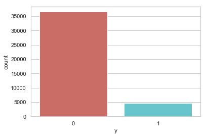
data['y'].value_counts()
0    36548
1     4640
Name: y, dtype: int64
sns.countplot(x='y', data = data, palette='hls')
plt.show()
plt.savefig('count_plot')
<Figure size 432x288 with 0 Axes>
count_no_sub = len(data[data['y']==0])
count_sub = len(data[data['y']==1])
pct_of_no_sub = count_no_sub/(count_no_sub+count_sub)
print('未开户的百分比:  %.2f%%' % (pct_of_no_sub*100))
pct_of_sub = count_sub/(count_no_sub+count_sub)
print('开户的百分比:  %.2f%%' % (pct_of_sub*100))
未开户的百分比:  88.73%
开户的百分比:  11.27%
data.groupby('y').mean()
| age | duration | campaign | pdays | previous | emp_var_rate | cons_price_idx | cons_conf_idx | euribor3m | nr_employed | |
|---|---|---|---|---|---|---|---|---|---|---|
| y | ||||||||||
| 0 | 39.911185 | 220.844807 | 2.633085 | 984.113878 | 0.132374 | 0.248875 | 93.603757 | -40.593097 | 3.811491 | 5176.166600 |
| 1 | 40.913147 | 553.191164 | 2.051724 | 792.035560 | 0.492672 | -1.233448 | 93.354386 | -39.789784 | 2.123135 | 5095.115991 |
观察:
购买定期存款的客户的平均年龄高于未购买定期存款的客户的平均年龄。
购买定期存款的客户的 pdays(自上次联系客户以来的日子)较低。 pdays越低,最后一次通话的记忆越好,因此销售的机会就越大。
令人惊讶的是,购买定期存款的客户的销售通话次数较低。
我们可以计算其他特征值(如教育和婚姻状况)的分布,以更详细地了解我们的数据。
data.groupby('job').mean()
| age | duration | campaign | pdays | previous | emp_var_rate | cons_price_idx | cons_conf_idx | euribor3m | nr_employed | y | |
|---|---|---|---|---|---|---|---|---|---|---|---|
| job | |||||||||||
| admin. | 38.187296 | 254.312128 | 2.623489 | 954.319229 | 0.189023 | 0.015563 | 93.534054 | -40.245433 | 3.550274 | 5164.125350 | 0.129726 |
| blue-collar | 39.555760 | 264.542360 | 2.558461 | 985.160363 | 0.122542 | 0.248995 | 93.656656 | -41.375816 | 3.771996 | 5175.615150 | 0.068943 |
| entrepreneur | 41.723214 | 263.267857 | 2.535714 | 981.267170 | 0.138736 | 0.158723 | 93.605372 | -41.283654 | 3.791120 | 5176.313530 | 0.085165 |
| housemaid | 45.500000 | 250.454717 | 2.639623 | 960.579245 | 0.137736 | 0.433396 | 93.676576 | -39.495283 | 4.009645 | 5179.529623 | 0.100000 |
| management | 42.362859 | 257.058140 | 2.476060 | 962.647059 | 0.185021 | -0.012688 | 93.522755 | -40.489466 | 3.611316 | 5166.650513 | 0.112175 |
| retired | 62.027326 | 273.712209 | 2.476744 | 897.936047 | 0.327326 | -0.698314 | 93.430786 | -38.573081 | 2.770066 | 5122.262151 | 0.252326 |
| self-employed | 39.949331 | 264.142153 | 2.660802 | 976.621393 | 0.143561 | 0.094159 | 93.559982 | -40.488107 | 3.689376 | 5170.674384 | 0.104856 |
| services | 37.926430 | 258.398085 | 2.587805 | 979.974049 | 0.154951 | 0.175359 | 93.634659 | -41.290048 | 3.699187 | 5171.600126 | 0.081381 |
| student | 25.894857 | 283.683429 | 2.104000 | 840.217143 | 0.524571 | -1.408000 | 93.331613 | -40.187543 | 1.884224 | 5085.939086 | 0.314286 |
| technician | 38.507638 | 250.232241 | 2.577339 | 964.408127 | 0.153789 | 0.274566 | 93.561471 | -39.927569 | 3.820401 | 5175.648391 | 0.108260 |
| unemployed | 39.733728 | 249.451677 | 2.564103 | 935.316568 | 0.199211 | -0.111736 | 93.563781 | -40.007594 | 3.466583 | 5157.156509 | 0.142012 |
| unknown | 45.563636 | 239.675758 | 2.648485 | 938.727273 | 0.154545 | 0.357879 | 93.718942 | -38.797879 | 3.949033 | 5172.931818 | 0.112121 |
data.groupby('marital').mean()
| age | duration | campaign | pdays | previous | emp_var_rate | cons_price_idx | cons_conf_idx | euribor3m | nr_employed | y | |
|---|---|---|---|---|---|---|---|---|---|---|---|
| marital | |||||||||||
| divorced | 44.899393 | 253.790330 | 2.61340 | 968.639853 | 0.168690 | 0.163985 | 93.606563 | -40.707069 | 3.715603 | 5170.878643 | 0.103209 |
| married | 42.307165 | 257.438623 | 2.57281 | 967.247673 | 0.155608 | 0.183625 | 93.597367 | -40.270659 | 3.745832 | 5171.848772 | 0.101573 |
| single | 33.158714 | 261.524378 | 2.53380 | 949.909578 | 0.211359 | -0.167989 | 93.517300 | -40.918698 | 3.317447 | 5155.199265 | 0.140041 |
| unknown | 40.275000 | 312.725000 | 3.18750 | 937.100000 | 0.275000 | -0.221250 | 93.471250 | -40.820000 | 3.313038 | 5157.393750 | 0.150000 |
data.groupby('education').mean()
| age | duration | campaign | pdays | previous | emp_var_rate | cons_price_idx | cons_conf_idx | euribor3m | nr_employed | y | |
|---|---|---|---|---|---|---|---|---|---|---|---|
| education | |||||||||||
| Basic | 42.163910 | 263.043874 | 2.559498 | 974.877967 | 0.141053 | 0.191329 | 93.639933 | -40.927595 | 3.729654 | 5172.014113 | 0.087029 |
| high.school | 37.998213 | 260.886810 | 2.568576 | 964.358382 | 0.185917 | 0.032937 | 93.584857 | -40.940641 | 3.556157 | 5164.994735 | 0.108355 |
| illiterate | 48.500000 | 276.777778 | 2.277778 | 943.833333 | 0.111111 | -0.133333 | 93.317333 | -39.950000 | 3.516556 | 5171.777778 | 0.222222 |
| professional.course | 40.080107 | 252.533855 | 2.586115 | 960.765974 | 0.163075 | 0.173012 | 93.569864 | -40.124108 | 3.710457 | 5170.155979 | 0.113485 |
| university.degree | 38.879191 | 253.223373 | 2.563527 | 951.807692 | 0.192390 | -0.028090 | 93.493466 | -39.975805 | 3.529663 | 5163.226298 | 0.137245 |
| unknown | 43.481225 | 262.390526 | 2.596187 | 942.830734 | 0.226459 | 0.059099 | 93.658615 | -39.877816 | 3.571098 | 5159.549509 | 0.145003 |
%matplotlib inline
table=pd.crosstab(data.job,data.y)
table.div(table.sum(1).astype(float), axis=0).plot(kind='bar', stacked=True)
plt.title('Stacked Bar Chart of Job title vs Purchase')
plt.xlabel('Job')
plt.ylabel('Proportion of Purchase')
plt.savefig('purchase_vs_job')
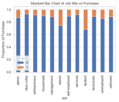
具有不同职位的人购买存款的频率不一样。 因此,职称可以是良好的预测因素。
table=pd.crosstab(data.marital,data.y)
table.div(table.sum(1).astype(float), axis=0).plot(kind='bar', stacked=True)
plt.title('Stacked Bar Chart of Marital Status vs Purchase')
plt.xlabel('Marital Status')
plt.ylabel('Proportion of Customers')
plt.savefig('mariral_vs_pur_stack')
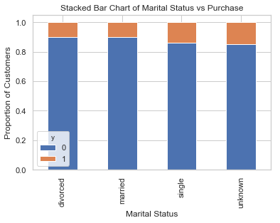
婚姻状况似乎不是好的预测因素。
table=pd.crosstab(data.education,data.y)
table.div(table.sum(1).astype(float), axis=0).plot(kind='bar', stacked=True)
plt.title('Stacked Bar Chart of Education vs Purchase')
plt.xlabel('Education')
plt.ylabel('Proportion of Customers')
plt.savefig('edu_vs_pur_stack')
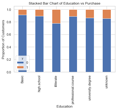
教育似乎是结果变量的良好预测指标。
table=pd.crosstab(data.day_of_week,data.y)#.plot(kind='bar')
table.div(table.sum(1).astype(float), axis=0).plot(kind='bar', stacked=True)
plt.title('Stacked Bar Chart of Day of Week vs Purchase')
plt.xlabel('Day of Week')
plt.ylabel('Proportion of Purchase')
plt.savefig('dow_vs_purchase')
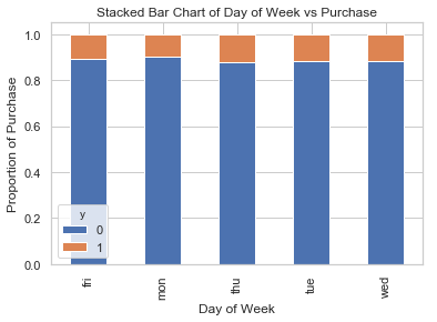
一周工作时间不是预测结果的良好预测因素。
cat_vars=['job','marital','education','default','housing','loan','contact','month','day_of_week','poutcome']
for var in cat_vars:
    cat_list = pd.get_dummies(data[var], prefix=var)
    data=data.join(cat_list)
data_final=data.drop(cat_vars, axis=1)
data_final.columns.values
array(['age', 'duration', 'campaign', 'pdays', 'previous', 'emp_var_rate',
       'cons_price_idx', 'cons_conf_idx', 'euribor3m', 'nr_employed', 'y',
       'job_admin.', 'job_blue-collar', 'job_entrepreneur',
       'job_housemaid', 'job_management', 'job_retired',
       'job_self-employed', 'job_services', 'job_student',
       'job_technician', 'job_unemployed', 'job_unknown',
       'marital_divorced', 'marital_married', 'marital_single',
       'marital_unknown', 'education_Basic', 'education_high.school',
       'education_illiterate', 'education_professional.course',
       'education_university.degree', 'education_unknown', 'default_no',
       'default_unknown', 'default_yes', 'housing_no', 'housing_unknown',
       'housing_yes', 'loan_no', 'loan_unknown', 'loan_yes',
       'contact_cellular', 'contact_telephone', 'month_apr', 'month_aug',
       'month_dec', 'month_jul', 'month_jun', 'month_mar', 'month_may',
       'month_nov', 'month_oct', 'month_sep', 'day_of_week_fri',
       'day_of_week_mon', 'day_of_week_thu', 'day_of_week_tue',
       'day_of_week_wed', 'poutcome_failure', 'poutcome_nonexistent',
       'poutcome_success'], dtype=object)
使用SMOTE进行过采样 创建我们的训练数据后,我将使用SMOTE算法(合成少数过采样技术)对已经开户的用户进行上采样。 在高层次上,SMOTE:
通过从次要类(已经开户的用户)创建合成样本而不是创建副本来工作。
随机选择一个k-最近邻居并使用它来创建一个类似但随机调整的新观察结果。
使用如下命令安装: conda install -c conda-forge imbalanced-learn
X = data_final.loc[:, data_final.columns != 'y']
y = data_final.loc[:, data_final.columns == 'y'].values.ravel()

from imblearn.over_sampling import SMOTE
os = SMOTE(random_state=0)
X_train, X_test, y_train, y_test = train_test_split(X, y, test_size=0.3, random_state=0)
columns = X_train.columns
os_data_X,os_data_y=os.fit_sample(X_train, y_train)
os_data_X = pd.DataFrame(data=os_data_X,columns=columns )
os_data_y= pd.DataFrame(data=os_data_y,columns=['y'])
# we can Check the numbers of our data
print("过采样以后的数据量: ",len(os_data_X))
print("未开户的用户数量: ",len(os_data_y[os_data_y['y']==0]))
print("开户的用户数量: ",len(os_data_y[os_data_y['y']==1]))
print("未开户的用户数量的百分比: ",len(os_data_y[os_data_y['y']==0])/len(os_data_X))
print("开户的用户数量的百分比: ",len(os_data_y[os_data_y['y']==1])/len(os_data_X))
过采样以后的数据量:  51134
未开户的用户数量:  25567
开户的用户数量:  25567
未开户的用户数量的百分比:  0.5
开户的用户数量的百分比:  0.5
现在我们拥有完美平衡的数据! 您可能已经注意到我仅对训练数据进行了过采样
from sklearn.linear_model import LogisticRegression
from sklearn import metrics
#X_train, X_test, y_train, y_test = train_test_split(X, y, test_size=0.3, random_state=0)
logreg = LogisticRegression()
logreg.fit(os_data_X, os_data_y.values.reshape(-1))
 LogisticRegression(C=1.0, class_weight=None, dual=False, fit_intercept=True,
          intercept_scaling=1, max_iter=100, multi_class='warn',
          n_jobs=None, penalty='l2', random_state=None, solver='warn',
          tol=0.0001, verbose=0, warm_start=False)
y_pred = logreg.predict(X_test)
print('在测试数据集上面的预测准确率: {:.2f}'.format(logreg.score(X_test, y_test)))
在测试数据集上面的预测准确率: 0.86
from sklearn.metrics import classification_report
print(classification_report(y_test, y_pred))
              precision    recall  f1-score   support

           0       0.98      0.86      0.92     10981
           1       0.44      0.88      0.59      1376

   micro avg       0.86      0.86      0.86     12357
   macro avg       0.71      0.87      0.75     12357
weighted avg       0.92      0.86      0.88     12357
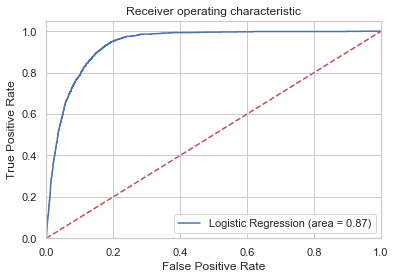
from sklearn.metrics import roc_auc_score
from sklearn.metrics import roc_curve
logit_roc_auc = roc_auc_score(y_test, logreg.predict(X_test))
fpr, tpr, thresholds = roc_curve(y_test, logreg.predict_proba(X_test)[:,1])
plt.figure()
plt.plot(fpr, tpr, label='Logistic Regression (area = %0.2f)' % logit_roc_auc)
plt.plot([0, 1], [0, 1],'r--')
plt.xlim([0.0, 1.0])
plt.ylim([0.0, 1.05])
plt.xlabel('False Positive Rate')
plt.ylabel('True Positive Rate')
plt.title('Receiver operating characteristic')
plt.legend(loc="lower right")
plt.savefig('Log_ROC')
plt.show()
2.预测Titanic乘客是否能在事故中生还
import numpy as np
import pandas as pd

from sklearn import preprocessing
import matplotlib.pyplot as plt
plt.rc("font", size=14)
import seaborn as sns
sns.set(style="white") #设置seaborn画图的背景为白色
sns.set(style="whitegrid", color_codes=True)
# 将数据读入 DataFrame
df = pd.read_csv("./titanic_data.csv")

# 预览数据
df.head()
| pclass | survived | name | sex | age | sibsp | parch | ticket | fare | cabin | embarked | |
|---|---|---|---|---|---|---|---|---|---|---|---|
| 0 | 1.0 | 1.0 | Allen, Miss. Elisabeth Walton | female | 29.0000 | 0.0 | 0.0 | 24160 | 211.3375 | B5 | S |
| 1 | 1.0 | 1.0 | Allison, Master. Hudson Trevor | male | 0.9167 | 1.0 | 2.0 | 113781 | 151.5500 | C22 C26 | S |
| 2 | 1.0 | 0.0 | Allison, Miss. Helen Loraine | female | 2.0000 | 1.0 | 2.0 | 113781 | 151.5500 | C22 C26 | S |
| 3 | 1.0 | 0.0 | Allison, Mr. Hudson Joshua Creighton | male | 30.0000 | 1.0 | 2.0 | 113781 | 151.5500 | C22 C26 | S |
| 4 | 1.0 | 0.0 | Allison, Mrs. Hudson J C (Bessie Waldo Daniels) | female | 25.0000 | 1.0 | 2.0 | 113781 | 151.5500 | C22 C26 | S |
df.shape
(1310, 11)
print('数据集包含的数据个数 {}.'.format(df.shape[0]))
数据集包含的数据个数 1310.
# 查看数据集中各个特征缺失的情况
df.isnull().sum()
pclass         1
survived       1
name           1
sex            1
age          264
sibsp          1
parch          1
ticket         1
fare           2
cabin       1015
embarked       3
dtype: int64
# "age" 缺失的百分比
print('"age" 缺失的百分比  %.2f%%' %((df['age'].isnull().sum()/df.shape[0])*100))
"age" 缺失的百分比 20.15%
约 20% 的乘客的年龄缺失了. 看一看年龄的分别情况.
ax = df["age"].hist(bins=15, color='teal', alpha=0.6)
ax.set(xlabel='age')
plt.xlim(-10,85)
plt.show()
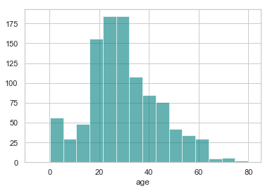
由于“年龄”的偏度不为0, 使用均值替代缺失值不是最佳选择, 这里可以选择使用中间值替代缺失值
<font color=red> 注: 在概率论和统计学中,偏度衡量实数随机变量概率分布的不对称性。偏度的值可以为正,可以为负或者甚至是无法定义。在数量上,偏度为负(负偏态)就意味着在概率密度函数左侧的尾部比右侧的长,绝大多数的值(不一定包括中位数在内)位于平均值的右侧。偏度为正(正偏态)就意味着在概率密度函数右侧的尾部比左侧的长,绝大多数的值(不一定包括中位数)位于平均值的左侧。偏度为零就表示数值相对均匀地分布在平均值的两侧,但不一定意味着其为对称分布。</font>
# 年龄的均值
print('The mean of "Age" is %.2f' %(df["age"].mean(skipna=True)))
# 年龄的中间值
print('The median of "Age" is %.2f' %(df["age"].median(skipna=True)))
The mean of "Age" is 29.88
The median of "Age" is 28.00
# 仓位缺失的百分比
print('"Cabin" 缺失的百分比 %.2f%%' %((df['cabin'].isnull().sum()/df.shape[0])*100))
"Cabin" 缺失的百分比 77.48%
约 77% 的乘客的仓位都是缺失的, 最佳的选择是不使用这个特征的值.
# 登船地点的缺失率
print('"Embarked" 缺失的百分比 %.2f%%' %((df['embarked'].isnull().sum()/df.shape[0])*100))
"Embarked" 缺失的百分比 0.23%
只有 0.23% 的乘客的登船地点数据缺失, 可以使用众数替代缺失的值.
print('按照登船地点分组 (C = Cherbourg, Q = Queenstown, S = Southampton):')
print(df['embarked'].value_counts())
sns.countplot(x='embarked', data=df, palette='Set2')
plt.show()
按照登船地点分组 (C = Cherbourg, Q = Queenstown, S = Southampton):
S    914
C    270
Q    123
Name: embarked, dtype: int64
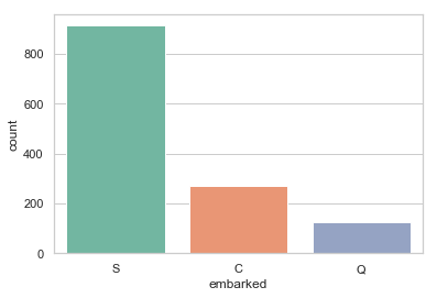
print('乘客登船地点的众数为 %s.' %df['embarked'].value_counts().idxmax())
乘客登船地点的众数为 S.
由于大多数人是在南安普顿(Southhampton)登船, 可以使用“S”替代缺失的数据值
根据缺失数据情况调整数据:
- 如果一条数据的 “Age” 缺失, 使用年龄的中位数 28 替代.
- 如果一条数据的 “Embarked” 缺失, 使用登船地点的众数 “S” 替代.
- 由于太多乘客的 “Cabin” 数据缺失, 从所有数据中丢弃这个特征的值.
data = df.copy()
data["age"].fillna(df["age"].median(skipna=True), inplace=True)
data["embarked"].fillna(df['embarked'].value_counts().idxmax(), inplace=True)
data.drop('cabin', axis=1, inplace=True)
# 确认数据是否还包含缺失数据
data.isnull().sum()
pclass      1
survived    1
name        1
sex         1
age         0
sibsp       1
parch       1
ticket      1
fare        2
embarked    0
dtype: int64
其他缺失的数据用其众数替代
data["pclass"].fillna(df['pclass'].value_counts().idxmax(), inplace=True)
data["survived"].fillna(df['survived'].value_counts().idxmax(), inplace=True)
data["name"].fillna(df['name'].value_counts().idxmax(), inplace=True)
data["sex"].fillna(df['sex'].value_counts().idxmax(), inplace=True)
data["sibsp"].fillna(df['sibsp'].value_counts().idxmax(), inplace=True)
data["parch"].fillna(df['parch'].value_counts().idxmax(), inplace=True)
data["ticket"].fillna(df['ticket'].value_counts().idxmax(), inplace=True)
data["fare"].fillna(df['fare'].value_counts().idxmax(), inplace=True)
# 预览调整过的数据
data.head()
| pclass | survived | name | sex | age | sibsp | parch | ticket | fare | embarked | |
|---|---|---|---|---|---|---|---|---|---|---|
| 0 | 1.0 | 1.0 | Allen, Miss. Elisabeth Walton | female | 29.0000 | 0.0 | 0.0 | 24160 | 211.3375 | S |
| 1 | 1.0 | 1.0 | Allison, Master. Hudson Trevor | male | 0.9167 | 1.0 | 2.0 | 113781 | 151.5500 | S |
| 2 | 1.0 | 0.0 | Allison, Miss. Helen Loraine | female | 2.0000 | 1.0 | 2.0 | 113781 | 151.5500 | S |
| 3 | 1.0 | 0.0 | Allison, Mr. Hudson Joshua Creighton | male | 30.0000 | 1.0 | 2.0 | 113781 | 151.5500 | S |
| 4 | 1.0 | 0.0 | Allison, Mrs. Hudson J C (Bessie Waldo Daniels) | female | 25.0000 | 1.0 | 2.0 | 113781 | 151.5500 | S |
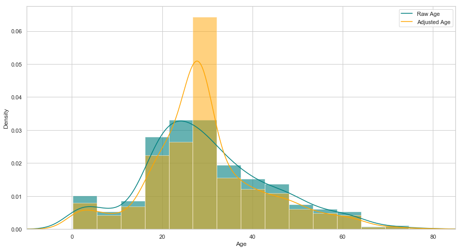
# 查看年龄在调整前后的分布
plt.figure(figsize=(15,8))
ax = df["age"].hist(bins=15, normed=True, stacked=True, color='teal', alpha=0.6)
df["age"].plot(kind='density', color='teal')
ax = data["age"].hist(bins=15, normed=True, stacked=True, color='orange', alpha=0.5)
data["age"].plot(kind='density', color='orange')
ax.legend(['Raw Age', 'Adjusted Age'])
ax.set(xlabel='Age')
plt.xlim(-10,85)
plt.show()
其它特征的处理
数据中的两个特征 “sibsp” (一同登船的兄弟姐妹或者配偶数量)与“parch”(一同登船的父母或子女数量)都是代表是否有同伴同行. 为了预防这两个特征具有多重共线性, 我们可以将这两个变量转为一个变量 “TravelAlone” (是否独自一人成行)
注: 多重共线性(multicollinearity)是指多变量线性回归中,变量之间由于存在高度相关关系而使回归估计不准确。比如虚拟变量陷阱(英语:Dummy variable trap)即有可能触发多重共线性问题。## 创建一个新的变量'TravelAlone'记录是否独自成行, 丢弃“sibsp” (一同登船的兄弟姐妹或者配偶数量)与“parch”(一同登船的父母或子女数量)
data['TravelAlone']=np.where((data["sibsp"]+data["parch"])>0, 0, 1)
data.drop('sibsp', axis=1, inplace=True)
data.drop('parch', axis=1, inplace=True)
对类别变量(categorical variables)使用独热编码(One-Hot Encoding), 将字符串类别转换为数值
# 对 Embarked","Sex"进行独热编码, 丢弃 'name', 'ticket'
final =pd.get_dummies(data, columns=["embarked","sex"])
final.drop('name', axis=1, inplace=True)
final.drop('ticket', axis=1, inplace=True)

final.head()
| pclass | survived | age | fare | TravelAlone | embarked_C | embarked_Q | embarked_S | sex_female | sex_male | |
|---|---|---|---|---|---|---|---|---|---|---|
| 0 | 1.0 | 1.0 | 29.0000 | 211.3375 | 1 | 0 | 0 | 1 | 1 | 0 |
| 1 | 1.0 | 1.0 | 0.9167 | 151.5500 | 0 | 0 | 0 | 1 | 0 | 1 |
| 2 | 1.0 | 0.0 | 2.0000 | 151.5500 | 0 | 0 | 0 | 1 | 1 | 0 |
| 3 | 1.0 | 0.0 | 30.0000 | 151.5500 | 0 | 0 | 0 | 1 | 0 | 1 |
| 4 | 1.0 | 0.0 | 25.0000 | 151.5500 | 0 | 0 | 0 | 1 | 1 | 0 |
数据分析
# 年龄
plt.figure(figsize=(15,8))
ax = sns.kdeplot(final["age"][final.survived == 1], color="darkturquoise", shade=True)
sns.kdeplot(final["age"][final.survived == 0], color="lightcoral", shade=True)
plt.legend(['Survived', 'Died'])
plt.title('Density Plot of Age for Surviving Population and Deceased Population')
ax.set(xlabel='Age')
plt.xlim(-10,85)
plt.show()
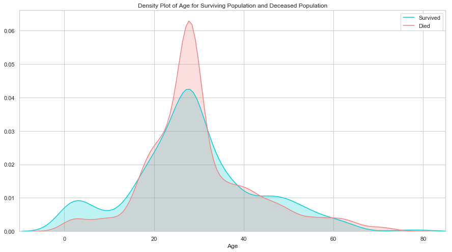
生还与遇难群体的分布相似, 唯一大的区别是生还群体中用一部分低年龄的乘客. 说明当时的人预先保留了孩子的生还机会.
# 票价
plt.figure(figsize=(15,8))
ax = sns.kdeplot(final["fare"][final.survived == 1], color="darkturquoise", shade=True)
sns.kdeplot(final["fare"][final.survived == 0], color="lightcoral", shade=True)
plt.legend(['Survived', 'Died'])
plt.title('Density Plot of Fare for Surviving Population and Deceased Population')
ax.set(xlabel='Fare')
plt.xlim(-20,200)
plt.show()
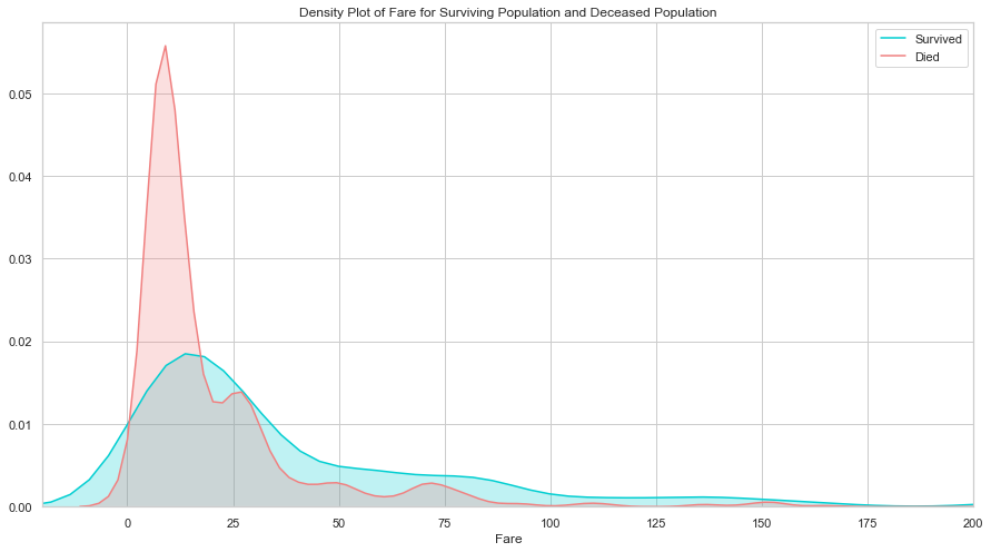
生还与遇难群体的票价分布差异比较大, 说明这个特征对预测乘客是否生还非常重要. 票价和仓位相关, 也许是仓位影响了逃生的效果, 我们接下来看仓位的分析.
# 仓位
sns.barplot('pclass', 'survived', data=df, color="darkturquoise")
plt.show()
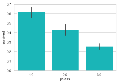
如我们所料, 一等舱的乘客生还几率最高.
# 登船地点
sns.barplot('embarked', 'survived', data=df, color="teal")
plt.show()
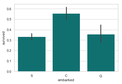
从法国 Cherbourge 登录的乘客生还率最高
# 是否独自成行
sns.barplot('TravelAlone', 'survived', data=final, color="mediumturquoise")
plt.show()
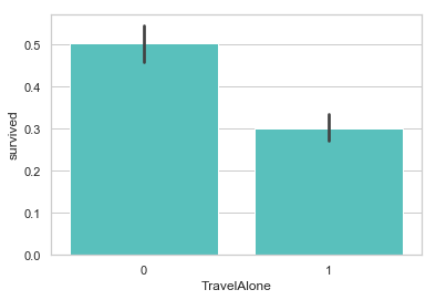
独自成行的乘客生还率比较低. 当时的年代, 大多数独自成行的乘客为男性居多.
# 性别
sns.barplot('sex', 'survived', data=df, color="aquamarine")
plt.show()
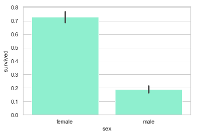
很明显, 女性的生还率比较高
# 使用Logistic Regression做预测
from sklearn.linear_model import LogisticRegression
from sklearn.model_selection import train_test_split
from sklearn.metrics import accuracy_score
from sklearn.preprocessing import StandardScaler

# 使用如下特征做预测
cols = ["age","fare","TravelAlone","pclass","embarked_C","embarked_S","sex_male"]

# 创建 X (特征) 和 y (类别标签)
X = final[cols]
y = final['survived']

# 将 X 和 y 分为两个部分
X_train, X_test, y_train, y_test = train_test_split(X, y, test_size=0.2, random_state=2)


# 检测 logistic regression 模型的性能
# DONE 添加代码:
# 1.训练模型,


# 特征缩放
# X_normalizer = StandardScaler() # N(0,1)
# X_train = X_normalizer.fit_transform(X_train)
# X_test = X_normalizer.transform(X_test)

logreg = LogisticRegression()
logreg.fit(X_train, y_train)


# 2.根据模型, 以 X_test 为输入, 生成变量 y_pred

y_pred = logreg.predict(X_test)

print('Train/Test split results:')
print("准确率为 %2.3f" % accuracy_score(y_test, y_pred))
Train/Test split results:
准确率为 0.828
多项逻辑回归
逻辑回归与最大熵
逻辑回归本质上是一种最大熵模型。它们都是求条件概率分布下样本数据的对数似然最大化。