KNN核心思想
K最近邻算法是指:在给定的训练数据(样本)集中,对于新的输入样本,通过计算新样本与所有训练样本的距离,找到与新样本最近的K个训练样本(K个邻居),对于分类问题,K个训练样本中属于某类标签的个数最多,就把新样本分到那个标签类别中,对于回归问题,将K个训练样本的目标值的均值作为新样本的目标值。
KNN只有待调整(确定)的超参数K,没有待学习的模型参数。
超参数K可通过交叉验证(cross validation)来确定。具体地,先将待学习的数据集分为训练数据(train)和测试数据(test),再将训练数据进一步训练数据(training data)和验证数据(validation data),选择不同K的情况下,验证数据中系统性能指标最好的那个超参数K。
对于5-Fold 交叉验证,可将原有的训练数据分为5等份,每次选其中一份作为验证集,其他四份作为训练集,可做5次。将每次得到的系统指标(准确率)取平均作为最终的某个K时的系统指标。
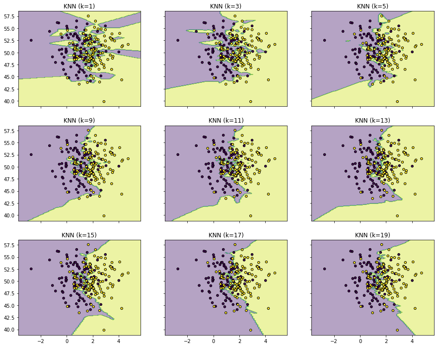
随着K的增加,RNN的决策边界越来越平滑。
说明: 交叉验证只是起到增大数据量的目的,不用交叉验证,直接用全量的训练数据也可以确定超参数K。
注意事项
- 不同维度特征的数值不要相差过大,否则在计算距离时,会导致某一维度的特征不起作用。可利用线性归一化(min-max normalization)[$x_{new}=\frac{x-\min \left( x \right)}{\max \left( x \right) -\min \left( x \right)}$]或标准差标准化(z-score normalization)[$x_{new}=\frac{x-mean\left( x \right)}{std\left( x \right)}$]进行特征缩放
- 对于大数据量的训练数据集,当样本维度不大时,可以采用KD-tree的数据结构来提高计算效率;当样本维度较大时,采用 Locality Sensitivity Hashing (LSH)的近似算法提高效率(将距离比较近的样本以较大的概率放到同一个bucket里)
- 在计算距离时,可考虑两个样本点间的相关性。可利用 Mahalanobis Distance($d_M\left( x_1,x_2 \right) =\left( x_1-x_2 \right) ^TM\left( x_1-x_2 \right) $,其中$M$为待学习的参数矩阵)进行距离的计算。具体可参考论文Distance Metric Learning for Large Margin Nearest Neighbor Classification
- 在K个样本中可以考虑不同样本与新样本的权重,不只看不同类别样本的个数,也叫weighted KNN
- 引入kernel trick,kernelized KNN
优点
- 算法简单
- 比较适合用在低维空间
- 可作为baseline
缺点
- 因需要计算新样本与所有训练样本的距离,复杂度高,对大数据量需要一定的处理
- 不适合高维特征
KNN实战
鸢尾花(iris)的分类
调用KNN函数来实现分类
数据采用的是经典的iris数据,是三分类问题
# 读取相应的库
from sklearn import datasets
from sklearn.model_selection import train_test_split
from sklearn.neighbors import KNeighborsClassifier
import numpy as np
# 读取数据 X, y
iris = datasets.load_iris()
X = iris.data
y = iris.target
print(X[:5])
print(y)
[[5.1 3.5 1.4 0.2]
 [4.9 3.  1.4 0.2]
 [4.7 3.2 1.3 0.2]
 [4.6 3.1 1.5 0.2]
 [5.  3.6 1.4 0.2]]
[0 0 0 0 0 0 0 0 0 0 0 0 0 0 0 0 0 0 0 0 0 0 0 0 0 0 0 0 0 0 0 0 0 0 0 0 0
 0 0 0 0 0 0 0 0 0 0 0 0 0 1 1 1 1 1 1 1 1 1 1 1 1 1 1 1 1 1 1 1 1 1 1 1 1
 1 1 1 1 1 1 1 1 1 1 1 1 1 1 1 1 1 1 1 1 1 1 1 1 1 1 2 2 2 2 2 2 2 2 2 2 2
 2 2 2 2 2 2 2 2 2 2 2 2 2 2 2 2 2 2 2 2 2 2 2 2 2 2 2 2 2 2 2 2 2 2 2 2 2
 2 2]
# 把数据分成训练数据和测试数据
X_train, X_test, y_train, y_test = train_test_split(X, y, random_state=2003)
# 构建KNN模型, K值为3、 并做训练
clf = KNeighborsClassifier(n_neighbors=3)
clf.fit(X_train, y_train)
KNeighborsClassifier(algorithm='auto', leaf_size=30, metric='minkowski',
           metric_params=None, n_jobs=None, n_neighbors=3, p=2,
           weights='uniform')
# 计算准确率
from sklearn.metrics import accuracy_score
# correct = np.count_nonzero((clf.predict(X_test)==y_test)==True)
print("Accuracy is: %.3f" % accuracy_score(y_test, clf.predict(X_test)))
# print ("Accuracy is: %.3f" %(correct/len(X_test)))
Accuracy is: 0.921
从零开始自己写一个KNN算法
from sklearn import datasets
from collections import Counter  # 为了做投票
from sklearn.model_selection import train_test_split
import numpy as np

# 导入iris数据
iris = datasets.load_iris()
X = iris.data
y = iris.target
X_train, X_test, y_train, y_test = train_test_split(X, y, random_state=2003)
def euc_dis(instance1, instance2):
    """
    计算两个样本instance1和instance2之间的欧式距离
    instance1: 第一个样本, array型
    instance2: 第二个样本, array型
    """
    # TODO
    dist = np.sqrt(sum((instance1 - instance2)**2))
    return dist


def knn_classify(X, y, testInstance, k):
    """
    给定一个测试数据testInstance, 通过KNN算法来预测它的标签。
    X: 训练数据的特征
    y: 训练数据的标签
    testInstance: 测试数据,这里假定一个测试数据 array型
    k: 选择多少个neighbors?
    """
    # TODO  返回testInstance的预测标签 = {0,1,2}
    distances = [euc_dis(x, testInstance) for x in X]
    kneighbors = np.argsort(distances)[:k]
    count = Counter(y[kneighbors])
    return count.most_common()[0][0]
# 预测结果。
predictions = [knn_classify(X_train, y_train, data, 3) for data in X_test]
correct = np.count_nonzero((predictions==y_test)==True)
#print("Accuracy is: %.3f" % accuracy_score(y_test, clf.predict(X_test)))
print ("Accuracy is: %.3f" %(correct/len(X_test)))
Accuracy is: 0.921
KNN的决策边界
import matplotlib.pyplot as plt
import numpy as np
from itertools import product
from sklearn.neighbors import KNeighborsClassifier

# 生成一些随机样本
n_points = 100
X1 = np.random.multivariate_normal([1,50], [[1,0],[0,10]], n_points)
X2 = np.random.multivariate_normal([2,50], [[1,0],[0,10]], n_points)
X = np.concatenate([X1,X2])
y = np.array([0]*n_points + [1]*n_points)
print (X.shape, y.shape)
(200, 2) (200,)
# KNN模型的训练过程
clfs = []
neighbors = [1,3,5,9,11,13,15,17,19]
for i in range(len(neighbors)):
    clfs.append(KNeighborsClassifier(n_neighbors=neighbors[i]).fit(X,y))
# 可视化结果
x_min, x_max = X[:, 0].min() - 1, X[:, 0].max() + 1
y_min, y_max = X[:, 1].min() - 1, X[:, 1].max() + 1
xx, yy = np.meshgrid(np.arange(x_min, x_max, 0.1),
                     np.arange(y_min, y_max, 0.1))

f, axarr = plt.subplots(3,3, sharex='col', sharey='row', figsize=(15, 12))
for idx, clf, tt in zip(product([0, 1, 2], [0, 1, 2]),
                        clfs,
                        ['KNN (k=%d)'%k for k in neighbors]):
    Z = clf.predict(np.c_[xx.ravel(), yy.ravel()])
    Z = Z.reshape(xx.shape)

    axarr[idx[0], idx[1]].contourf(xx, yy, Z, alpha=0.4)
    axarr[idx[0], idx[1]].scatter(X[:, 0], X[:, 1], c=y,
                                  s=20, edgecolor='k')
    axarr[idx[0], idx[1]].set_title(tt)

plt.show()
二手车价格的预测
import pandas as pd
import matplotlib
import matplotlib.pyplot as plt
import numpy as np
import seaborn as sns
#读取数据
df = pd.read_csv('data.csv')
df  # data frame
| Brand | Type | Color | Construction Year | Odometer | Ask Price | Days Until MOT | HP | |
|---|---|---|---|---|---|---|---|---|
| 0 | Peugeot 106 | 1.0 | blue | 2002 | 166879 | 999 | 138 | 60 |
| 1 | Peugeot 106 | 1.0 | blue | 1998 | 234484 | 999 | 346 | 60 |
| 2 | Peugeot 106 | 1.1 | black | 1997 | 219752 | 500 | -5 | 60 |
| 3 | Peugeot 106 | 1.1 | red | 2001 | 223692 | 750 | -87 | 60 |
| 4 | Peugeot 106 | 1.1 | grey | 2002 | 120275 | 1650 | 356 | 59 |
| 5 | Peugeot 106 | 1.1 | red | 2003 | 131358 | 1399 | 266 | 60 |
| 6 | Peugeot 106 | 1.1 | green | 1999 | 304277 | 799 | 173 | 57 |
| 7 | Peugeot 106 | 1.4 | green | 1998 | 93685 | 1300 | 0 | 75 |
| 8 | Peugeot 106 | 1.1 | white | 2002 | 225935 | 950 | 113 | 60 |
| 9 | Peugeot 106 | 1.4 | green | 1997 | 252319 | 650 | 133 | 75 |
| 10 | Peugeot 106 | 1.0 | black | 1998 | 220000 | 700 | 82 | 50 |
| 11 | Peugeot 106 | 1.1 | black | 1997 | 212000 | 700 | 75 | 60 |
| 12 | Peugeot 106 | 1.1 | black | 2003 | 255134 | 799 | 197 | 60 |
#清洗数据
# 把颜色独热编码
df_colors = df['Color'].str.get_dummies().add_prefix('Color: ')
# 把类型独热编码
df_type = df['Type'].apply(str).str.get_dummies().add_prefix('Type: ')
# 添加独热编码数据列
df = pd.concat([df, df_colors, df_type], axis=1)
# 去除独热编码对应的原始列
df = df.drop(['Brand', 'Type', 'Color'], axis=1)

df
| Construction Year | Odometer | Ask Price | Days Until MOT | HP | Color: black | Color: blue | Color: green | Color: grey | Color: red | Color: white | Type: 1.0 | Type: 1.1 | Type: 1.4 | |
|---|---|---|---|---|---|---|---|---|---|---|---|---|---|---|
| 0 | 2002 | 166879 | 999 | 138 | 60 | 0 | 1 | 0 | 0 | 0 | 0 | 1 | 0 | 0 |
| 1 | 1998 | 234484 | 999 | 346 | 60 | 0 | 1 | 0 | 0 | 0 | 0 | 1 | 0 | 0 |
| 2 | 1997 | 219752 | 500 | -5 | 60 | 1 | 0 | 0 | 0 | 0 | 0 | 0 | 1 | 0 |
| 3 | 2001 | 223692 | 750 | -87 | 60 | 0 | 0 | 0 | 0 | 1 | 0 | 0 | 1 | 0 |
| 4 | 2002 | 120275 | 1650 | 356 | 59 | 0 | 0 | 0 | 1 | 0 | 0 | 0 | 1 | 0 |
| 5 | 2003 | 131358 | 1399 | 266 | 60 | 0 | 0 | 0 | 0 | 1 | 0 | 0 | 1 | 0 |
| 6 | 1999 | 304277 | 799 | 173 | 57 | 0 | 0 | 1 | 0 | 0 | 0 | 0 | 1 | 0 |
| 7 | 1998 | 93685 | 1300 | 0 | 75 | 0 | 0 | 1 | 0 | 0 | 0 | 0 | 0 | 1 |
| 8 | 2002 | 225935 | 950 | 113 | 60 | 0 | 0 | 0 | 0 | 0 | 1 | 0 | 1 | 0 |
| 9 | 1997 | 252319 | 650 | 133 | 75 | 0 | 0 | 1 | 0 | 0 | 0 | 0 | 0 | 1 |
| 10 | 1998 | 220000 | 700 | 82 | 50 | 1 | 0 | 0 | 0 | 0 | 0 | 1 | 0 | 0 |
| 11 | 1997 | 212000 | 700 | 75 | 60 | 1 | 0 | 0 | 0 | 0 | 0 | 0 | 1 | 0 |
| 12 | 2003 | 255134 | 799 | 197 | 60 | 1 | 0 | 0 | 0 | 0 | 0 | 0 | 1 | 0 |
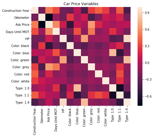
# 数据转换
matrix = df.corr()
f, ax = plt.subplots(figsize=(8, 6))
sns.heatmap(matrix, square=True)
plt.title('Car Price Variables')
Text(0.5, 1.0, 'Car Price Variables')
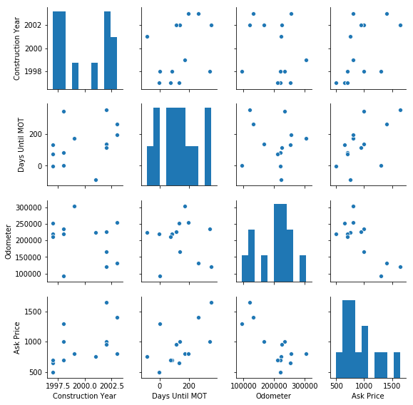
# 不同维度特征间的关系图
sns.pairplot(df[['Construction Year', 'Days Until MOT', 'Odometer', 'Ask Price']], size=2)
plt.show()
from sklearn.neighbors import KNeighborsRegressor
from sklearn.model_selection import train_test_split
from sklearn import preprocessing
from sklearn.preprocessing import StandardScaler
import numpy as np

X = df[['Construction Year', 'Days Until MOT', 'Odometer']]
y = df['Ask Price'].values.reshape(-1, 1)
X_train, X_test, y_train, y_test = train_test_split(X, y, test_size=0.3, random_state=41)

# 特征缩放
X_normalizer = StandardScaler() # N(0,1)
X_train = X_normalizer.fit_transform(X_train)
X_test = X_normalizer.transform(X_test)

y_normalizer = StandardScaler()
y_train = y_normalizer.fit_transform(y_train)
y_test = y_normalizer.transform(y_test)

# 训练拟合
knn = KNeighborsRegressor(n_neighbors=2)
knn.fit(X_train, y_train.ravel())

# Now we can predict prices:
y_pred = knn.predict(X_test)
# 反向缩放,还原实际的量纲

# 预测的值
y_pred_inv = y_normalizer.inverse_transform(y_pred)
# 真实的值
y_test_inv = y_normalizer.inverse_transform(y_test)

# Build a plot
plt.scatter(y_pred_inv, y_test_inv)
plt.xlabel('Prediction')
plt.ylabel('Real value')

# Now add the perfect prediction line
diagonal = np.linspace(500, 1500, 100)
plt.plot(diagonal, diagonal, '-r')
plt.xlabel('Predicted ask price')
plt.ylabel('Ask price')
plt.show()

print('Prediction',y_pred_inv)
print('Real value',y_test_inv)
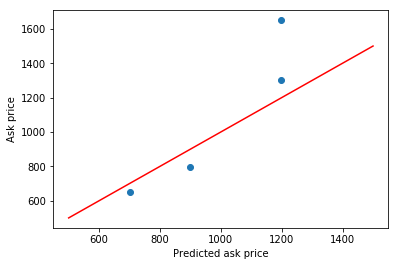
Prediction [1199. 1199.  700.  899.]
Real value [[1300.]
 [1650.]
 [ 650.]
 [ 799.]]